-
Notifications
You must be signed in to change notification settings - Fork 2
CIRN Digital Earth Australia Coastal Earth Observation Workshop

Stephen Sagar - Assistant Director, Coastal & Aquatic Earth Observation Science
Robbi Bishop-Taylor - Coastal Earth Observation Scientist
We will be using the Digital Earth Australia Sandbox analysis environment for this workshop. The DEA Sandbox is an interactive Python-based coding environment with access to petabytes of satellite data across Australia and pre-installed scientific Python packages for EO analysis.
-
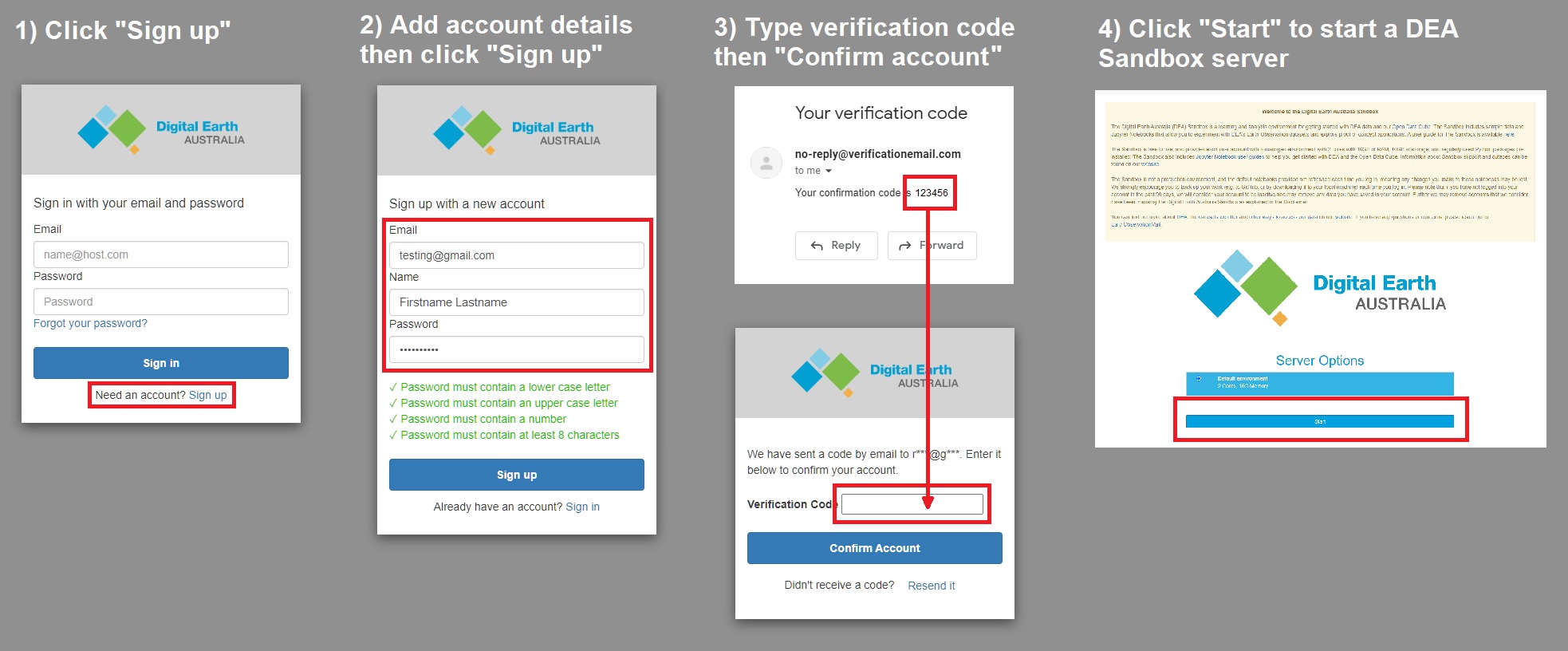
Please follow the guide here to register for the DEA Sandbox before the Tuesday morning workshop: https://knowledge.dea.ga.gov.au/guides/setup/Sandbox/sandbox/#register
Important
Once you have registered, email Robbi.BishopTaylor@ga.gov.au if you would like to be granted access to larger 120 gb RAM, 16 CPUs resources during the workshop!
- Additional Sandbox resources are provided for the purposes of this workshop for a period of six weeks
- After six weeks (30th November 2024), access will revert to the default provisions
- When you have finished using the DEA Sandbox, please shut down your server by clicking the
Filemenu, thenHub control panelthenStop my server.

eo-tides is a new coastal remote sensing Python package that provides parallelized tools for integrating satellite Earth observation data with tide modelling. eo-tides combines advanced tide modelling functionality from the pyTMD package with pandas, xarray and odc-geo, providing a suite of flexible tools for efficient analysis of coastal and ocean Earth observation data – from regional, continental, to global scale.
These tools can be applied to petabytes of freely available satellite data (e.g. from Digital Earth Australia or Microsoft Planetary Computer) loaded via Open Data Cube's odc-stac or datacube packages, supporting coastal and ocean earth observation analysis for any time period or location globally.
Follow the instructions below to get started with eo-tides on the DEA Sandbox:
-
Log into the DEA Sandbox (https://app.sandbox.dea.ga.gov.au/):

-
Start up a server - select "4XL environment for coastal modelling workshop" if you emailed about extra access; otherwise "Default Environment":

-
Press "Start" and wait for your server to launch. This may take several minutes.

-
After a few minutes, your Sandbox will launch and you should see the screen below. On the left is a file browser that you can use to navigate the Sandbox. On the right is a window where we will run interactive "Jupyter Notebook" code examples (for more information, see here).

-
On the top-left, you will see a blue "New launcher" button. Click this, and then click "Start a new terminal session"


-
The
eo-tidescode and examples live on Github here (https://github.com/GeoscienceAustralia/eo-tides). Our first step is to get a copy ofeo-tidesinside the DEA Sandbox so we can run it interactively. The commands below will create a "clone" of theeo-tidesrepository, and then installeo-tidesas a Python package so we can use it:Clone
eo-tidesinto a newCIRN/eo-tides/directory:git clone https://github.com/GeoscienceAustralia/eo-tides.git CIRN/eo-tidesAnd now install
eo-tides:pip install eo-tidesWe are now ready to get started!
-
Using the file browser menu on the left, navigate to
CIRN > eo-tides > docs > notebooks. You will see a list of "Jupyter Notebook" files:
-
Double click on
Model_tides.ipynbto launch our first Jupyter Notebook:
-
Jupyter Notebooks are interactive code examples that contain a mixture of static documentation text, and interactive code. To interact with the notebook, click on any cell, then either click the "play" button above to run the code, or shift-enter on your keyboard.

The
[ ]:symbol to the left of each Code cell describes the state of the cell:-
[ ]:means that the cell has not been run yet. -
[*]:means that the cell is currently running. -
[1]:means that the cell has finished running and was the first cell run.
-
-
By default, our Jupyter Notebook comes with outputs from the previous run included in the file. As a first step, we're going to restart and clear our notebook so we can start from fresh. Click
Kernelin the file menu up the top-left, then clickRestart Kernel and clear all outputs of all cells. This will restart the notebook and clear all our outputs.
Tip
If you ever get stuck, you can restart your Jupyter Notebook by running Kernel > Restart Kernel and clear all outputs of all cells at any time.
This workshop session will demonstrate how to use the model_tides function from the eo_tides.model module to model tide heights at multiple coordinates or time steps, using one or multiple ocean tide models.
The model_tides function supports tide modelling based on a wide range of ocean tide models using a single line of code, parallelising this modelling where possible and returning data in a standardised pandas.Dataframe format.
The model_tides function can be used independently of Earth observation (EO) data, e.g. for any application where you need to generate a time series of tide heights.
However, it also underpins the more complex EO-related functions demonstrated in Combining tides with satellite data.
Getting started:
-
Important: the first step in an
eo-tidesanalysis is to download and set up tide models. We have set up the DEA Sandbox with some models for you, but we still need to telleo-tideswhere these files are located. In the code cell below, update the code fromdirectory = "../../tests/data/tide_models/"to:directory = "/var/share/tide_models/"
-
We've now set up the notebook ready to run. Follow along with the workshop presenter, running each cell one-by-one (using the "play" button or shift-enter) as instructed.
Open satellite data repositories like Digital Earth Australia, Microsoft Planetary Computer and Element84 Earth Search and global metadata standards like SpatioTemporal Asset Catalogue make it easier than ever to load satellite data for anywhere on the planet. Combining this satellite data with tide modelling can be a powerful approach for correcting coastal imagery and for better understanding coastal processes captured by EO data.
This workshop session will demonstrate how to load free and open satellite data for anywhere on the planet using odc-stac, and then combine that satellite data with tide modelling using the tag_tides and pixel_tides functions from eo_tides.eo. These functions allow you to model the height of the tide at the exact moment of satellite image acquisition, and analyse satellite EO data by tidal conditions - for example, filter your data to satellite imagery collected during specific tidal stages (e.g. low or high tide).
Getting started:
-
In the file browser menu, double-click on
Satellite_data.ipynbto launch our second Jupyter Notebook:
-
Perform a
Kernel > Restart Kernel and clear all outputs of all cellsto clear the notebook for a fresh start -
As in the previous example, to access our tide models we first need to update the code under "Getting started" from
directory = "../../tests/data/tide_models/"to:directory = "/var/share/tide_models/" -
We've now set up the notebook ready to run. Follow along with the workshop presenter, running each cell one-by-one (using the "play" button or shift-enter) as instructed.
Complex interactions between temporal tide dynamics and the regular mid-morning overpass timing of sun-synchronous sensors like Landsat or Sentinel-2 mean that satellites often does not observe the entire tidal cycle. Biases in satellite coverage of the tidal cycle can mean that tidal extremes (e.g. the lowest or highest tides at a location) may either never be captured by satellites, or be over-represented in the satellite EO record. Local tide dynamics can cause these biases to vary greatly both through time and spatially, making it challenging to consistently analyse and compare coastal processes consistently - particularly for large-scale regional or global analyses.
To ensure that coastal EO analyses are not inadvertently affected by tide biases, it is important to compare how well the tides observed by satellites match the full range of tides at a location. This session will demonstrate how to use the tide_stats and pixel_stats functions from eo_tides.stats to calculate local tide statistics and identify biases caused by interactions between tidal processes and satellite orbits.
Getting started:
-
In the file browser menu, double-click on
Tide_statistics.ipynbto launch our third Jupyter Notebook:
-
Perform a
Kernel > Restart Kernel and clear all outputs of all cellsto clear the notebook for a fresh start -
As in the previous example, to access our tide models we first need to update the code under "Getting started" from
directory = "../../tests/data/tide_models/"to:directory = "/var/share/tide_models/" -
We've now set up the notebook ready to run. Follow along with the workshop presenter, running each cell one-by-one (using the "play" button or shift-enter) as instructed.
The intertidal zone (i.e. the land along the coast that is periodically inundated by the tide) support important ecological habitats (e.g. sandy beaches and shores, tidal flats and rocky shores and reefs), and provide many valuable benefits such as storm surge protection, carbon storage and natural resources for recreational and commercial use. However, intertidal zones are faced with increasing threats from coastal erosion, land reclamation (e.g. port construction), and sea level rise. Accurate mapping data describing the spatial extents of the intertidal zone are essential for managing these environments, and predicting when and where these threats will have the greatest impact. However, the intertidal zone is challenging and expensive to map at large scale using intensive manual survey methods - particularly across large coastal regions.
Freely available satellite EO data provides a powerful and cost-effective tool for mapping the intertidal zone at regional, national scale or global scale. This session will demonstrate a simple intertidal mapping workflow that combines free and open Landsat satellite data with tide modelling from eo-tides. This workflow can be adapted to explore different tidal conditions, study areas or sensors.
Getting started:
-
In the file browser menu, double-click on
Case_study_intertidal.ipynbto launch our fourth Jupyter Notebook:
-
Perform a
Kernel > Restart Kernel and clear all outputs of all cellsto clear the notebook for a fresh start -
As in the previous example, to access our tide models we first need to update the code under "Getting started" from
directory = "../../tests/data/tide_models/"to:directory = "/var/share/tide_models/" -
In this more complex case study example, we also have some additional configurable parameters under Analysis parameters. However, don't change these parameters on your first run - we can return and change them once we have finished running the notebook from start to finish!

-
We've now set up the notebook ready to run. Follow along with the workshop presenter, running each cell one-by-one (using the "play" button or shift-enter) as instructed.
-
Once you have finished running the notebook, you can download the
intertidal_map.tifintertidal map classification we generated to your PC so that you can explore it in a GIS software like QGIS. Right-click onintertidal_map.tifin the file browser menu on the left of the DEA Sandbox, and click "Download":
Tip
If you would like to try running this or any other Jupyter Notebook outside of Australia, you can find global-coverage EOT20 tide model data at the following location:
directory = "/var/share/tide_models/global/"
- Clone DEA Intertidal repo:
git clone https://github.com/GeoscienceAustralia/dea-intertidal.git CIRN/dea-intertidal
-
Launch and run
CIRN/dea-intertidal/notebooks/Intertidal_elevation_stac.ipynbJupyter Notebook -
Choose a location on the interactive map (< 500 km2 recommended)
-
Follow the remainder of the notebook instructions to generate an intertidal DEM!

