DNN separation mechanisms

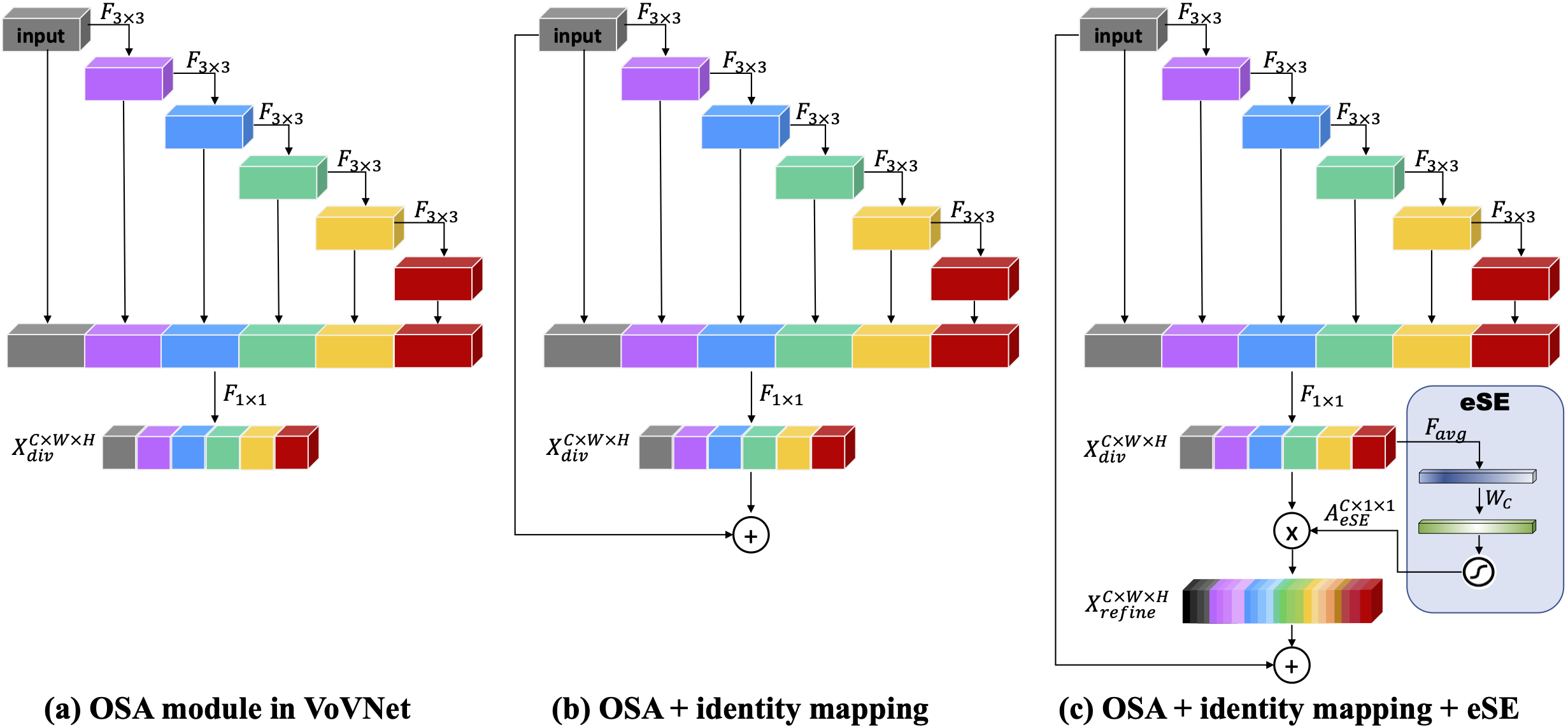
The implementation mechanisms of some neural networks are actually quite simple, but the use of numerous modules and complex structures makes it difficult to analyze the essence. Here, I plan to extract and organize some of the more central modules to reduce the burden on researchers

---

1. Transform-Average-Concatenate (TAC) module implementation

• reference: https://github.com/yoonsanghyu/FaSNet-TAC-PyTorch

---

2. DeepFiltering

• Including: DfOp and MultiframeOP
• reference https://github.com/Rikorose/DeepFilterNet

---

3. OSA_RES_eSE

• reference https://github.com/youngwanLEE/vovnet-detectron2

4. Difussion Method

In this context, it seems that separation is not related. However, if we consider the distribution of learning from a perspective, there may also need to understand here. Maybe you can understand me as being forced to explain. But I hope to use simple ways to explain the implementation process of code so that it helps understanding. All about SDEs.

4.1 Forward Process

• Perturbed_data

  In the given case of x, y and t, how do we generate an intermediate perturbed data? This is the most core content.

---

• step1 -- sample a t. To avoid some numerical errors, the minimum value of t should be greater than 0.03. This is an empirical value
• step2 -- get mean and std. In this process, there are many ways to compute mean and variance, but the most central point is to design well a path. With the path in hand, mean and variance become samples on the path.
• step3 -- get Perturbed_data. In both SDE or diffusion equation's understanding, the perturbed data here is a deterministic sample based on mean and variance.

Anthor thing is the loss. err = score * sigmas + z.

From intuition, model ignores the mean part of input and pre-dictes a noise with lower intensity compared to current noise by multiplying the square root of variance.

4.2 Sampling process

Here I quote from the paper about PC Sampler for better explanation.

Firstly, prior sampling is required. Add noise to y and the standard deviation of the noise is equal to the noise strength at the end of the additive process

'''python def prior_sampling(self, shape, y): if shape != y.shape: warnings.warn(f"Target shape {shape} does not match shape of y {y.shape}! Ignoring target shape.") std = self._std(torch.ones((y.shape[0],), device=y.device)) x_T = y + torch.randn_like(y) * std[:, None, None, None] return x_T '''

• PC_sampler

'''python def pc_sampler(): """The PC sampler function.""" with torch.no_grad(): xt = sde.prior_sampling(y.shape, y).to(y.device) timesteps = torch.linspace(sde.T, eps, sde.N, device=y.device) for i in range(sde.N): t = timesteps[i] vec_t = torch.ones(y.shape[0], device=y.device) * t xt, xt_mean = corrector.update_fn(xt, vec_t, y) xt, xt_mean = predictor.update_fn(xt, vec_t, y) x_result = xt_mean if denoise else xt ns = sde.N * (corrector.n_steps + 1) return x_result, ns

return pc_sampler

'''

• Correctors

  Currently I understand two kinds of correctors, one is Langevin Corrector and another is annealed Langevin Dynamics.

  SGMSE algorithm4

• Predictor

  Euler method

  diffusion reverse method

• v-Predictor